GGPlot Snippets

This is a collection of plots I find myself making often using data from CO2 and mtcars. The tidyverse package is assumed to be loaded, and other packages needed are explcitly shown in code.

Colors

By overall:

CO2 %>% ggplot(aes(conc,uptake,col=Treatment)) + geom_point() +
  scale_color_manual(values = c("red","green"))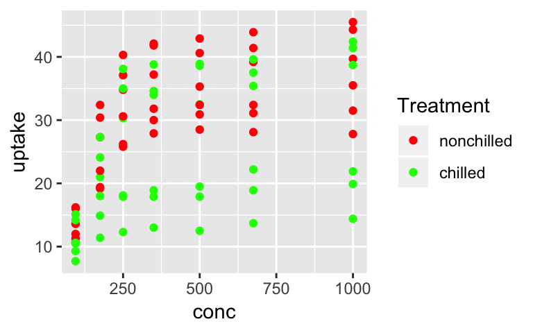

Categories in order unless specified:

data(CO2)
CO2 %>% ggplot(aes(conc,uptake,col=Treatment)) + geom_point() +
  scale_color_manual(values = c("chilled"="red","nonchilled"="green"))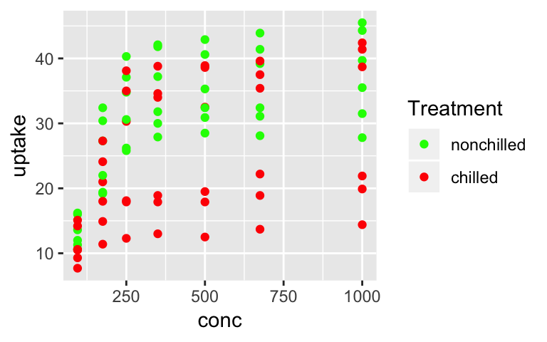

GGplot default:

CO2 %>% ggplot(aes(conc,uptake,col=Treatment)) + geom_point() +
  scale_color_manual(values = c("#F8766D","#00BFC4"))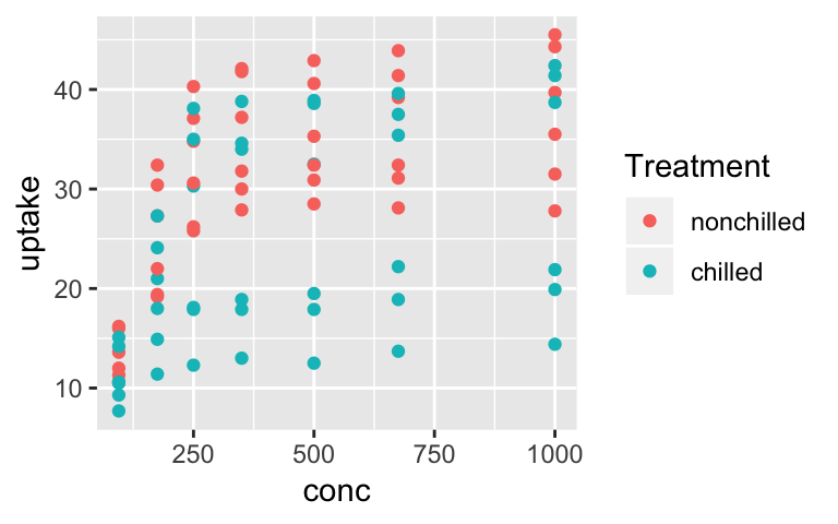

Brewer palette:

CO2 %>% ggplot(aes(conc,uptake,col=Treatment)) + geom_point() +
  scale_color_brewer(palette = "Dark2")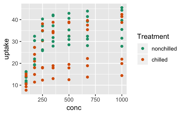

Type of scale: seq, div, qual

CO2 %>% ggplot(aes(conc,uptake,col=Treatment)) + geom_point() +
  scale_color_brewer(type="seq",direction = 1)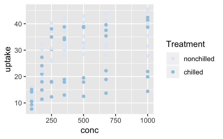 

Gradient:

CO2 %>% ggplot(aes(conc,uptake,col=conc)) + geom_point() +
  scale_color_gradient(low="blue", high="red")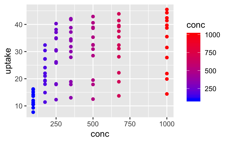

Keep levels even if not in subset plotted:

CO2 %>% filter(Treatment == "chilled") %>%
  ggplot(aes(conc,uptake,col=Treatment)) + geom_point() +
  scale_color_manual(values = c("#F8766D","#00BFC4"),drop  = FALSE)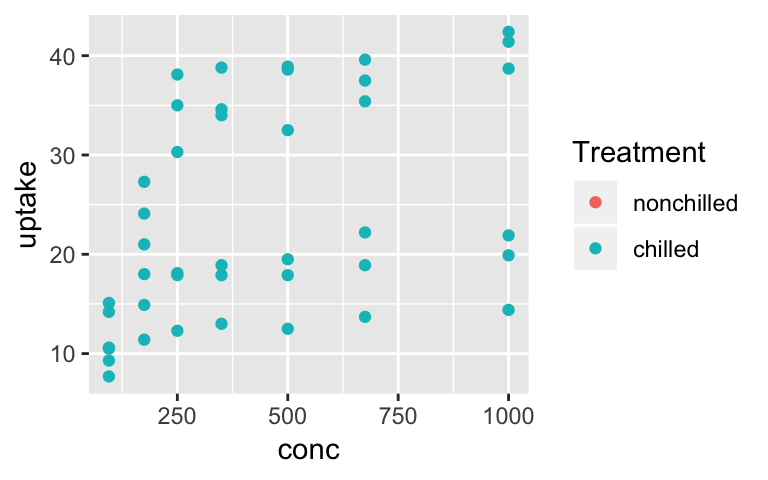

More info at http://www.sthda.com/english/wiki/ggplot2-colors-how-to-change-colors-automatically-and-manually

Comprehensive tutorial: http://zevross.com/blog/2014/08/04/beautiful-plotting-in-r-a-ggplot2-cheatsheet-3/

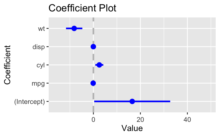
Plot of regression coefficients

library(coefplot)
data("mtcars")
m1 = glm(am == 1 ~ mpg + cyl + disp  + wt, data = mtcars, family = "binomial") %>% 
  coefplot() %>% 
  print()